gibson:teaching:spring-2018:math445:lecture:cylinderflow
Math 445 lecture 22: inviscid flow past a cylinder
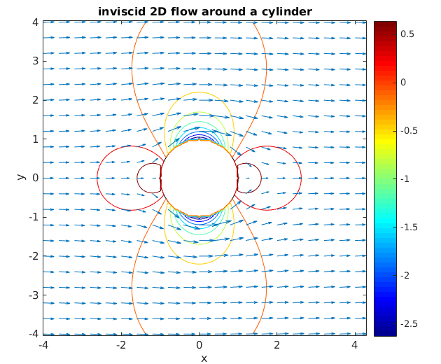
The velocity and pressure fields of inviscid, irrotational flow past a cylinder are given by

where  is the speed of the incoming fluid,
  is the radius of the cylinder centered at the origin, and
  are the polar coordinates of point
  .
These functions are valid only for points outside the cylinder
.
These functions are valid only for points outside the cylinder  .
.
The following Matlab code plots the velocity as a quiver plot and the pressure with contours.
- plotcylinderflow.m
%%%%%%%%%%%%%%%%%%%%%%%%%%%%%%%%%%%%%%%%%%%%%%%%%%%%%%%%%%%%%%%%%%
% Inviscid, irrotational flow around a cylinder
% Make quiver plot of velocity and contour plot of pressure for

% Vx(r,theta) =  V0 (1 - a^2/R^2 cos(2 theta))
% Vy(r,theta) = -V0 a^2/r^2 sin(2 theta)
%  p(r,theta) =   2 a^2/r^2 cos(2 theta) - a^4/r^4;

% for a=1, V0=1, on domain -4 <= x <= 4, -4 <= x <= 4

%%%%%%%%% Define constants %%%%%%%%%
V0 = 1;
a  = 1;

%%%%%%%%% First draw the cylinder %%%%%%%%%

theta = linspace(0, 2*pi, 100);
plot(a*cos(theta), a*sin(theta), 'k-')
hold on


%%%%%%%%% Second make the contour plot of pressure %%%%%%%%%

% define grid
x = linspace(-4,4,201); % contour plots need fine grids, so use lots of points
y = linspace(-4,4,201);
[X,Y] = meshgrid(x,y);

% compute polar coords r, theta on the x,y gridpoints
R = sqrt(X.^2 + Y.^2);
Theta = atan2(Y,X);     % use atan2(y,x) to get correct quadrant for theta

% evaluate the formula for the pressure field
P = (2*a^2)./R.^2 .* cos(2*Theta) - a.^4./R.^4;

% set P to zero inside the cylinder
P = (R > a) .* P;

% draw the contour plot, using ten contour lines
contour(x,y,P, 10);

colorbar
colormap jet

%%%%%%%%% Third make the quiver plot of velocity %%%%%%%%%

x = linspace(-4,4,21);  % quiver plots work better on coarse grids
y = linspace(-4,4,21);
[X,Y] = meshgrid(x,y);

R = sqrt(X.^2 + Y.^2);
Theta = atan2(Y,X);

% evaluate the formula for the velocity field
Vx = V0*(1 - a^2./R.^2 .* cos(2*Theta));
Vy = - V0*a^2./R.^2 .* sin(2*Theta);

% set Vx, Vy to zero inside the cylinder
Vx = (R > a) .* Vx;
Vy = (R > a) .* Vy;

% draw the quiver plot
quiver(x,y, Vx, Vy);

hold off

axis equal
axis tight

xlabel('x');
ylabel('y');
title('inviscid 2D flow around a cylinder')
gibson/teaching/spring-2018/math445/lecture/cylinderflow.txt · Last modified: 2018/04/10 06:52 by gibson
Except where otherwise noted, content on this wiki is licensed under the following license: CC Attribution-Share Alike 3.0 Unported
