Problem 1. Write numerical simulation for the heat eqn on a periodic domain using Fourier spatial discretization and Crank-Nicolson temporal discretization. Verify that your code works correctly by simulating the Gaussian-decay solution

from t = 1 to 100 for parameters , Lx=100, dt=1/16, Nx=128 (number of x gridpoints). Initialize your numerical code with u(x,1) and then compare the results of the numerical time integration with u(x,t) evaluated from the above formula. I suggest plotting both quantities versus x at regular intervals in time during the simulation, using “pause” (matlab) to stop the simulation temporarily.

Make a plot of the numerical solution and the Gaussian solution versus x at t=100 to turn in. Are the two entirely consistent? If not, why not?

Problem 2. Copy and revise your heat equation code so that it simulated the 1d Swift-Hohenberg equation, on a periodic domain using Fourier spatial discretization and Crank-Nicolson/Adams-Bashforth semi-implicit temporal discretization. Use the initial condition where , parameter values r = 0.2, Lx = 100, Nx = 256 (number of x gridpoints), dt = 1/16, and integrate from t=0 to 100.

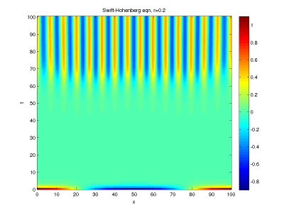
Make a colorplot of in the plane (using every x gridpoint but plotting t at a larger interval than dt, perhaps at intervals of 1/2 or 1. It should look something like this

When you are satisfied with the correctness of your simulation, make a plot of versus x for the above parameters and initial conditions to turn in.

Now play around with the forcing parameter in the range 0 < r < 1 and the initial condition, by changing the wavelengths and magnitudes of the the cosines, and possibly the total integration time, if you don't see patterns develop by t=100. Answer the following questions

1. Does the wavelength of the final pattern depend on r or the initial condition?
2. Does the wavelength of the final pattern match you expectation from linear analysis?
3. Can you relate the amplitude of the final pattern or the time scale of its growth from the initial condition to the Swift-Hohenberg equation?

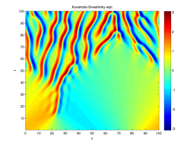
Problem 3. Copy and revise your Swift-Hohenberg code so that it simulates the 1d Kuramoto-Sivashinsky equation, , with parameters Lx = 100, Nx = 512, and dt = 1/16, initial condition (same as before), and integrate from t=0 to t=100. Make a colorplot of as before. It should look like this

Make a plot of versus x to turn in. Now play around with the domain size Lx (adjusting Nx so that Lx/Nx is approximately constant), try replacing the initial condition with random numbers of order 0.01, and answer the following questions

1. Does the wavelength of the final pattern depend on r or the initial condition?
2. Does the wavelength of the final pattern match you expectation from linear analysis?
3. What qualitative changes in behavior do you observe as L increases from small (L=1) to large (L=100)?

Problem 4. For each of the above codes, fix the initial condition and parameters, and run the simulation with dt = 1/8, 1/4, …. What happens? Why?

Some help on Matlab's FFT: Matlab documentation is not very helpful about the ordering or normalization of Fourier coefficients in the FFT. However, a small numerical experiment clarifies. Let's construct a function with energy in known wavenumbers and observe where nonzero coefficients appear in the numerical FFT. I'll do 8 gridpoints for the periodic domain [0, 2pi].

>> x = 1/8*(0:7)*2*pi
x =
         0    0.7854    1.5708    2.3562    3.1416    3.9270    4.7124    5.4978
  
>> k = 0; 
>> u = cos(k*x) + 0.1*sin(k*x);
>> [real(fft(u)); imag(fft(u))]
ans =
     8     0     0     0     0     0     0     0
     0     0     0     0     0     0     0     0


>> k = 1;
>> u = cos(k*x) + 0.1*sin(k*x);
>> [real(fft(u)); imag(fft(u))]
ans =
   -0.0000    4.0000    0.0000         0    0.0000         0    0.0000    4.0000
         0   -0.4000         0   -0.0000         0    0.0000         0    0.4000


>> k = 2;
>> u = cos(k*x) + 0.1*sin(k*x);
>> [real(fft(u)); imag(fft(u))]
ans =
   -0.0000   -0.0000    4.0000    0.0000    0.0000    0.0000    4.0000   -0.0000
         0         0   -0.4000         0         0         0    0.4000         0


>> k = 3;
>> u = cos(k*x) + 0.1*sin(k*x);
>> [real(fft(u)); imag(fft(u))]
ans =
   -0.0000    0.0000   -0.0000    4.0000    0.0000    4.0000   -0.0000    0.0000
         0   -0.0000    0.0000   -0.4000         0    0.4000   -0.0000    0.0000


>> k = 4;
>> u = cos(k*x) + 0.1*sin(k*x);
>> [real(fft(u)); imag(fft(u))]
ans =
         0         0         0         0    8.0000         0         0         0
         0    0.0000         0    0.0000         0   -0.0000         0   -0.0000

So the ordering of Fourier modes in the FFT for N=8 is k = [0 1 2 3 -4 -3 -2 -1] –not what I suggested it would be in class. The normalization is also different: the kth and -kth FFT coefficients for u(x) = cos(kx) are not 1/2, but N/2.

Also observe that the treatment of the highest-order Fourier mode k=-4 is a little weird, in that the 8 represents the sum of the k=4 and k=-4 cosine modes, with no representation of the k=4 and k=-4 sin modes. Without going into too much detail on this, Fourier spectral PDE codes typically just zero the highest-order mode at every time step. We can ignore this subtlety.

Based on the above, here's a short example of how to do Fourier differentiation in Matlab on a [0,L] periodic domain. This should be plenty to get you started for the time-stepping codes.

% A demonstration of Fourier differentiation in Matlab

% Parameters
L = 10;
N = 16;
x = L/N*(0:N-1);

% Set up u(x) and du/dx for some known L-periodic function
a = 2*pi/L
u    =   sin(a*x) + 0.2*cos(a*2*x);
dudx = a*cos(a*x) - 0.4*a*sin(a*2*x);

% Now compute dudx via FFT 
k = [0:N/2-1 -N/2:-1];
alpha = 2*pi*k/L;
D = i*alpha;  
dudx_fft = real(ifft(D.*fft(u)));

% Plot everybody
plot(x,u, 'b', x,dudx, 'g', x, dudx_fft, 'r.')
legend('u','du/dx','du/dx via FFT','location','southwest')
xlabel('x')