How to find invariant solutions

The channelflow findsoln utility will compute unstable equilibria, traveling waves, and (relative) periodic orbits of plane Couette or channel flows. Here are a few examples of usage.

periodic orbit of plane Couette flow

1. Generate a random velocity field with ''randomfield.''

randomfield -m 0.50 -lx 0.875 -lz 0.6 -Nx 32 -Ny 33 -Nz 32 u0

This will construct a random velocity field in file u0.h5, in a Lx x [-1, 1] x Lz periodic box with Lx = 2 lx pi = 1.75pi and Lz = 2 lz pi = 1.2 pi (the plane Couette minimal flow unit of Hamilton, Kim, Waleffe JFM 1995) with a 32 x 33 x 32 collocation grid (which is a lower resolution than I like for these calculations, but will result in a fast-running demo.) The velocity field u0 will be incompressible and have u=0 BCs at the wall, and will have an L2Norm of 0.50. You can check this by running fieldprops -n u0. I chose this magnitude for the field after testing some smaller fields and seeing that they died to laminar pretty quickly.

2. Integrate the random field forward in time.

couette -T1 1100 -dt 0.05 -R 400 -symms sxyz-sxytxz.asc u0.h5

This will time-integrate the field u0 as a perturbation on top of a laminar base flow U(y) = y for 1100 time units, at Re=400, and with time integration step dt=0.05, and enforcing symmetries in the velocity field specified by the file sxyz-sxytxz.asc By default the velocity field will be saved into a data directory at intervals dT=1. See integration for more information on time integration, such as the base flow plus fluctuation decomposition, or changing from plane Couette to channel conditions.

The symmetry file sxyz-sxytxz.asc has contents

% 2
 1 -1 -1 -1 0.0 0.0
 1 -1 -1  1 0.5 0.5

That specifies a symmetry group with two generators

$\begin{eqnarray*} \sigma_{xyz} : [u,v,w] (x,y,z) &\rightarrow [-u,-v,-w] (-x,-y,-z) \\ \sigma_{xy} \tau_{xz} : [u,v,w] (x,y,z) &\rightarrow [-u,-v,w] (-x+L_x/2,-y,z+L_z/2) \end{eqnarray*}$

The pointwise inversion $\sigma_{xyz}$ of this group fixes the origin and prevents traveling waves and arbitrary relative periodic orbits. For more on symmetry groups of plane Couette flow see symmetry and Gibson, Halcrow, Cvitanovic JFM 2009.

3. Select a good initial guess from a recurrence plot.

The $\langle \sigma_{xyz}, \sigma_{xy} \tau_{xz} \rangle$ symmetry group allows periodic orbits of the form $\tau u - f^T(u) = 0$ for $\tau \in \{i, \tau_x, \tau_z, \tau_{xz} \}$ , where $f^t$ is the forward-time evolution under Navier-Stokes, i.e. $u(t+T) = f^T(u(t))$ , and where $\tau_x$ represents a half-box shift in the $x$ direction, etc.

For this demo I'll just look for a solution of the form $u - f^T(u) = 0$ . Thus local minima of $\| u(t) - u(t+T) \|$ should provide good initial guesses for the search.

seriesdist -T0 0 -T1 1000 -dT 1 -tmax 100 -da data/ -db data/ -as -kx 8 -kz 8

This reads in the saved velocity fields from the data directory, computes $\| u(t) - u(t+T) \|$ as a function of $t,T$ , and saves this in the file dist.asc. Here's the recurrence plot for the data in question.

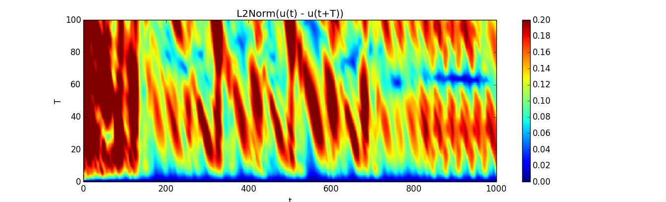
You can see strikingly periodic behavior over the range $825 \leq t \leq 1000$ with nice horizontal blue streak at $T \approx 65$ . This suggests the turbulent trajectory is shadowing a periodic orbit with period $T \approx 65$ . The minimum of $\| u(t) - u(t+T) \|$ in this region occurs at $t=917$ and $T=63$ . That's an unusually promising initial guess for a periodic orbit.

4. Find the periodic orbit with ''findsoln''

 
mkdir findsoln-917-63
cd findsoln-917-63
findsoln -orb -T 63 -dt 0.05 -R 400 -symms ../sxyz_sxytxz.asc ../data/u917.h5

Since I tend to run many searches for many initial guesses, I like to do each search in a subdirectory named after the initial guess. The findsoln command runs a Newton-Krylov-hookstep search that finds a $u,T$ solution of the equation $u - f^T(u) = 0$ given the initial guess $T=63$ and $u = u(917)$ . The search is restricted to the $\langle \sigma_{xyz}, \sigma_{xy} \tau_{xz} \rangle$ symmetry group. The symmetry restriction vastly reduces the search space and results in a faster and more robust search.

After about half an hour the search succeeds, finding a solution that satisfies the equation numerically to $O(10^{-13})$ . The characteristics of the search routine are recorded in the file convergence.asc

%-L2Norm(G)   r             delta         dT            L2Norm(du)    L2Norm(u)     L2Norm(dxN)   dxNalign      L2Norm(dxH)   GMRESerr      ftotal    fnewt     fhook     CFL       
0.00888606    2.20611e-05   0.01          0             0             0.390225      0             0             0             0             1         0         1         0.609524  
0.00663114    1.19704e-05   0.01          -0.0640999    0.0116139     0.38873       0.00902435    0             0.00902435    0.00076865    14        12        2         0.609524  
0.000855143   2.14948e-07   0.01          0.190862      0.00429167    0.388192      0.0548914     -0.238276     0.01          0.000119926   29        25        4         0.608904  
0.000597692   9.06641e-08   0.01          0.194443      0.00326027    0.387135      0.035679      0.998803      0.01          0.000613148   42        37        5         0.581667  
0.000505451   6.2892e-08    0.01          0.18166       0.00364325    0.386258      0.00942818    0.997453      0.00942818    0.000289388   55        49        6         0.583459  
1.77901e-05   8.04837e-11   0.01          -0.0438562    0.000824778   0.386507      0.00227387    -0.99388      0.00227387    0.000612772   67        60        7         0.604789  
5.46682e-09   8.266e-18     0.01          -0.000571434  1.73752e-05   0.38651       3.13122e-05   0.981989      3.13122e-05   5.95861e-05   80        72        8         0.584728  
8.51125e-13   1.58971e-25   0.01          -2.67003e-07  1.49819e-08   0.38651       1.70279e-08   0.940857      1.70279e-08   0.000134271   93        84        9         0.584723  
9.72014e-14   2.358e-27     0.01          -1.08282e-10  2.94411e-12   0.38651       5.77394e-12   0.921371      5.77394e-12   0.000331508   106       96        10        0.584723

The solution $u$ is stored in the file ubest.h5 and the value of $T$ in Tbest.asc.

channelflow.org

User Tools

Site Tools