Append the latest posts at the top of this page

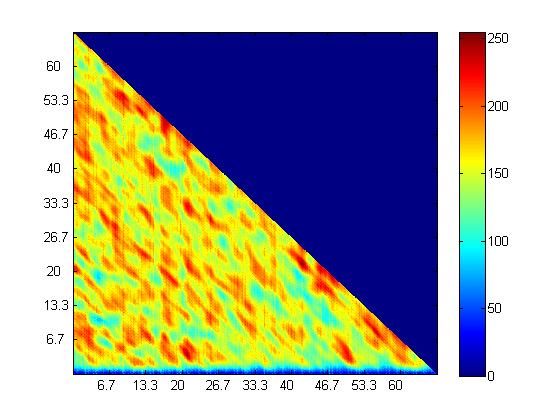
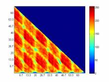
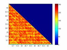
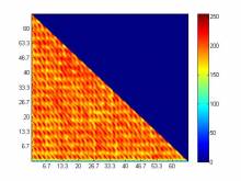
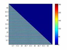
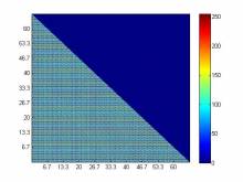
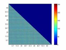
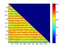
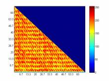
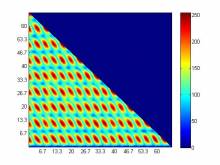
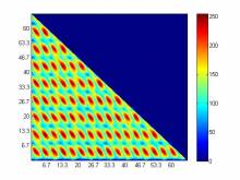
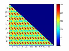
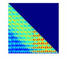
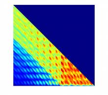
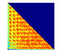
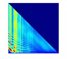
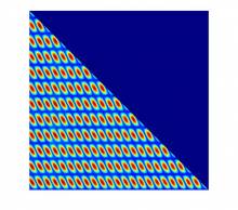
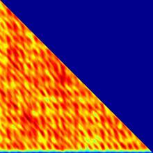
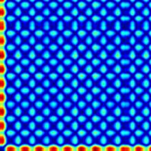
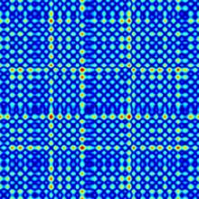
The following are recurrence plots for runs with DC current at 3V, 6V, 9V, 12V and 15V respectively:

The following videos correspond to the above plots:

3V: http://www.youtube.com/watch?v=HRbT2zgkMkg 6V: http://www.youtube.com/watch?v=BtSvv9C9HJI&feature=channel_page 9V: http://www.youtube.com/watch?v=44kXAITPM1A&feature=channel 12V: http://www.youtube.com/watch?v=s2VSBRYrpIU&feature=channel 15V: http://www.youtube.com/watch?v=SanCC1bl6hY&feature=channel

Here's a description of the experiment, currently in progress:

In general, we are investigating what is going on with forced two-dimensional turbulence. We have a thin layer of electrically conducting fluid on top of a bed of strong magnets, with glass separating the fluid and the magnets. Currently, the fluid is salt water. Then, we drive current through the water using two large electrodes hooked up to a power source and a function generator. The only signal we've tested thus far is a sine wave. The current goal is to find a regime of flow somewhere between periodic and turbulent motion.

Once we have enough preliminary data to know what we're actually looking for and what the parameters we'll be using are, we'll switch out the salt water for sulfuric acid, and make sure to keep the molarity consistent. We'll also be using a voltage to current converter so that we'll be keeping the current consistent rather than the voltage, which is what is more important.

We have a few different ways to look at data graphically right now. The first one is the velocity field data. Using particle image velocimetry software, we plug in a movie of the experiment into MATLAB and it spits out velocity field data, giving us an idea of which areas of the experiment have fluid moving in what direction. From velocity field data, we can make recurrence plots, which are what is plastered all over this blog. It's a scalar field that takes in the velocity field for two times, T + t and t, and finds the difference. The formula is Sum over velocity field of |U(T+t)-U(t)|. This will give a range of values, which is then assigned to different colors, and these colors are plotted on the recurrence plot. We can also make recurrence plots for individual vectors in the vector field. Recurrence plots appear to be “missing” the upper triangle of the graph - this is intentional, as there isn't actually any data in that region to be looked at. The horizontal axis is the t axis, and the vertical axis is the T axis. The units are in seconds. This allows us to spot periodicity better than a formula like |U(T)-U(t)|. The last way we are currently looking at data are time series, which are plots of the magnitude of a given vector or entire vector field over time.

Jon Paprocki 2009-03-26 2:18 PM

Explanation on what we're actually doing COMING SOON *cue movie preview music*

Short, temporary explanation: Put a thin layer of salt water on top of some strong magnets and drive current through it. Then, subject slave computer to hours of number crunching. Jon Paprocki 2009-02-24 11:13 AM

Can you start writing up the complete description of the experiment, in preparation for you term project report? Looking at it from Copenhagen I have no clue what is being measured (except that it looks cute) — Predrag Cvitanovic 2009-02-11 13:49

Here are movies of the .0625, .25, and .5 Hz runs mentioned below on the 03/26 post:

.0625 Hz video .0625 Hz velocity fields .25 Hz video .25 Hz velocity fields .5 Hz video .5 Hz velocity fields

After these movies I'm going to switch to uploading them here - I meant to do it for this batch but forgot and uploaded them to youtube out of habit.

Jon Paprocki 2009-03-26 1:53 PM

Movies of the first and third recurrence plots for the first search for something between periodic and turbulence motion posted to Schatz turbulence. It looks messy with lots of large conglomerates of glass spheres stuck together. We did 22 runs in a row and didn't want to change out the salt water since that would probably change the conductivity as well. It is also helpful since it shows that the PIV algorithm doesn't completely break when there is a lot of junk floating around.Jon Paprocki 2009-02-24 11:00 AM

Movies of the hybrid runs posted below are now up at Schatz turbulence. Jon Paprocki 2009-02-13 5:27 PM

Some of the preliminary 2-D turbulence movies and PIV data have been posted to Youtube at Schatz turbulence. While the movies look ok, the PIV vector fields did not survive the compression well, so if you want a better version please contact Jon Paprocki. — Daniel B. 2009-02-03 11:20

Things have been quiet on this page lately, but I haven't been slacking. We've been searching for a regime between periodic and turbulent flow, and here is the interesting stuff I've found in the last month.

These are recurrence plots of runs at 15 volts, with frequencies of .0625 Hz, .125 Hz, .25 Hz, .5 Hz, .75 Hz, and 1 Hz respectively.

You can see a very clear jump from vaguely semi-periodic to completely periodic motion between .25 and .5 Hz. .0625, .125, and .25 Hz all appear to be just plain turbulent to the naked eye, but the recurrence data suggests otherwise.

Also, I'm giving a talk on this project for the undergrad research symposium on April 1st in room 320 of the student center at 1:40 PM, if you're interested in something more detailed than this ramshackle blog.

EDIT: movies of these posted above in movies section

Jon Paprocki 2009-03-26 11:50 AM

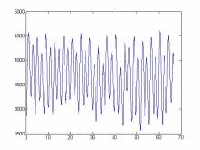
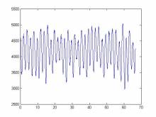
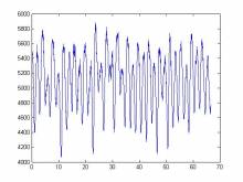
Recurrence plots for three higher voltages, with corresponding time series for the entire vector field. These are also at a new, slightly higher frequency. I don't know what the frequency was at before, but now the period of forcing is 3.92 seconds (for an entire cycle, so thats the time to go from +X to -X and back to +X).

Gotcha. That makes sense. If you expand out (sin(t+T) - sin(t))^2 you'll have some cos(t) and sin(t) mutliplicative factors that'll make r(t,T) oscillate in t.

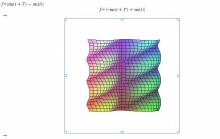
I think the behavior you're talking about on the recurrence plot being interesting is just natural for a recurrence plot of a periodic function. I tried making what I think ought to be the same thing as a recurrence plot in Maple by doing a 3D plot of |sin(t+T)-sin(t)| and it shows something that is qualitatively the same thing as these plots (though I have it flipped sideways).

Jon Paprocki 2009-02-20 2:18 PM

The units along the axes are in seconds. The period of forcing isn't really known, I've been told to not trust the frequency the signal generator claims it is making. I'll try hooking it up to an oscilloscope to find out what the actual frequency/period is and get back to you.

Mike pointed out that the plots still look mostly periodic - they do, but they definitely did not look like typical periodic motion in real life. I'll post movies of what happened with these plots by tuesday. Jon Paprocki 2009-02-20 1:41 PM

It is interesting that the recurrence plots r(t,T) = |u(t+T) - u(t)| are periodic in t as well as T. Some temporal phase of the periodic motion must be more coherent / less noisy than its quarter-period (?) temporal phase shift. By the way, what are the units of the time axes in these plots (seconds?) and what is the period of forcing in the same units? I don't know whether the periodicity in T of r(t,T) is half the forcing period or the full forcing period.

We did a search for something between periodic and turbulent motion. Here are a few of the recurrence plots:

These actually represent the three highest voltages we tried. We'll probably try higher voltages soon.

Jon Paprocki 2009-02-20 12:14 PM

Recurrence plots, now with time axes and color bar! I haven't looked up how to put this in the code instead of doing it manually, but I'll work that out on Tuesday. Here is what they should end up looking like:

Jon Paprocki 2009-02-13 4:59 PM

More recurrence plot data. Took 5 different runs trying different things. hybrid2 started at low voltage, and then jumped to a higher voltage about halfway through (so only two voltage levels total). hybrid3 ramped up the voltage every 10 seconds (6 times total). If you look closely, you can see the diagonals along which a voltage jump occured (or at least what I'm guessing is a result of it). hybrid4 slowly ramps up voltage continuously, starting at a very low voltage and ending at a medium voltage. hybrid5 slowly ramps up voltage continuously, starting where hybrid4 left off and ending very high. hybrid6 slowly ramps up frequency continuously at a constant medium voltage. I didn't expect hybrid6 to display much of anything, it started at less than 1 Hz and ended at something like 13 Hz according to the signal generator (which I've been told not to trust), but there is actually a very clear and obvious increase of frequency over time on the plot. I'll post movies of all of these runs and the velocity fields shortly.

hybrid2, hybrid3, hybrid4, hybrid5, hybrid6

Jon Paprocki 2009-02-13 3:18 PM

New recurrence plot data. turb3 shows what happens when we don't turn on the experiment for the first moment or so. Glassturb2 is interesting, because the motion looks somewhere between periodic and turbulent in the movie but looks relatively periodic in this data.

turb3, periodic3, and glassturb2

Jon Paprocki 2009-02-12 11:39 AM

Alright here is the new recurrence plot function. It takes awhile longer to run now, but its probably more accurate now too I'll figure out how I can work in some labels. I'll run the function on the other data sets we have on Thursday. I got rid of the fictitious data in the upper right triangle for the turbulent motion, but I ran the periodic data before I changed the code to not bother finding fictitious data. The function *should* now be working as John Gibson suggested. There are still some kinks to work out. The turbulent data would be more useful with some more variation in color. Daniel suggested charting it on a logarithmic scale. Edit: replaced periodic4 image with one without fictitious data 02/12/09

Periodic4 and Turb4:

Jon Paprocki 2009-02-10 1:46 PM

Could we flip the order of postings to make latest appear at the top? mfs 09022009 2:40

i agree with daniel's comment about labels for time units. however, i don't see how you can subtract off the periodic base flow…you need more than just the period of oscillation….you also need to know the amplitude of the periodic flow….how do we know that in the turbulent regime?

mfs 09022009 2:40

It would be nice to have some kind of time units on the axes of these recurrence plots and to know the driving frequency, so we could compare this to the apparent periodicity of the recurrence plots. It might also be helpful to subtract out the base periodic flow (although this might take some tinkering to get the phase right), so that only recurrences in the turbulent part of the flow show up. Right now, I think they might get blurred out by the recurrences due to the periodic forcing. — Daniel B. 2009-02-09 12:30

No problem, the information in the two plots should be the same. I just find the second easier to interpret at a glance. John Gibson 2009-02-07 5:39 PM

You're correct, that is what I ended up doing. Sleeping made me realize my mistake, because it was in my head when I woke up. I meant to do what you're saying! I'll get this fixed on Tuesday and post what it is supposed to be. Thanks! — Jon P. 2009-02-07 10:30 AM

Whoops! I didn't do what I thought I did. These aren't really recurrence plots! Or at least not in the sense that I thought they were. Jon Paprocki 2009-02-07 10:33 AM

Nice! Are you plotting r(t1, t2) = |u(t1)-u(t2)| where

? I have found I can spot good initial guesses for periodic orbits more easily if I look at plots of r(t,T) = |u(t+T) - u(t)|. Also, with symmetries it is helpful to look at r(t,T) = min_σ |σ u(t+T) - u(t)|, where σ ranges over the set of symmetries under which the relevant symmetric subspace is invariant. – John Gibson 2009-02-06 22:13

Here are some pictures of the recurrence plots. Both axes are time; the distance between two points along either axis is proportional to the time between the two points. Time “loops around” for the upper right triangle of each image (i.e. half of the image). The darker the color the closer in total vector magnitude the two points were. The lighter the color the further apart in total vector magnitude the two points were. I haven't yet analyzed the code close enough to make 100% sure that it's doing exactly what it's supposed to.

warning: the middle image of the turbulent motion collection is computed for a flow with large startup transients, so you can't conclude anything from this.

Turbulent motion:

Periodic motion:

— Jon P. 2009-02-06 6:28 PM

For future reference, since the number of MATLAB functions is quickly ballooning (and I'll lose track of it myself), here is how they are structured. I'll edit this as we go:

-Last Update 02/19/09

get_sample3.m → creates a bunch of files named file###.mat containing image info
-viewfiles.m → takes in a series of file###.mats and shows them on the screen as a movie
-pivCorrelate.m → takes in a series of file###.mats and outputs a correlation.mat file containing correlation data
–pivVelocityImages.m → takes in a correlation.mat file and outputs velocity field plots
–pivMagArray.m → takes in a correlation.mat file and outputs a magArray.mat file that contains the magnitudes of velocity vectors at every points
—pivTimeSeries.m → takes in a magArray.mat file and outputs a time series plot of the desired point
—pivTimeSeriesAll.m → same as pivTimeSeries, but sums the entire set of vectors in each frame instead of just one
–pivDifArray.m → takes in a correlation.mat file and outputs a difArray.mat that essentially is just converting the structure array of correlation.mat into a more usable array containing only the velocity data. This makes it easier to use vectorized code. This isn't the original use of the function so it isn't very aptly named…
—pivRecurrencePlot.m → takes in a difArray.mat file and outputs a recurrencePlot.mat file containing recurrence data.
—PivRecurrencePlotNew.m → uses the new formula for recurrence plots (doesn't square the difference vectors); outputs a recurrencePlotNew.mat file.
—-piv1DRecSlicet.m → grabs a “slice” of the recurrence plot at a given time along the t axis and plots it.
—-piv1DRecSliceTT.m → grabs a slice of the recurrence plot at a given time along the T axis and plots it.
—-minFinderY.m → “filters” out a recurrence plot by blotting out all the points that aren't minima along the Y axis, to some sensitivity.
—-minFinderX.m → same as minFinderY, but along the X axis.
—pivRecurrencePlotOne.m → same as pivRecurrence, but only does it for one specified point and ouputs a recurrenceDataLoc###.mat file
—-pivRecurrenceImage.m → takes in a recurrencePlot.mat or recurrenceDataLoc###.mat file and outputs an image of it.

— Jon Paprocki 2009-02-12 10:29 AM

Checked out Dustin and Jon Paprocki's permission problems on the wiki. Enabled gt2009 permissions for Jon P.; you should be able to start your own blog now. Jon P, your name is correct, but do you like Zappa? John Gibson 2009-02-04 12:12

John G. could you please give Jon Paprocki (he's the undergrad working on this project) access to the blog? Thanks – Daniel B. 2009-02-03 11:31