IAM 950 HW2
For this HW, you have a choice: compute periodic orbits of the Lorenz or the Rössler system. I demoed Lorenz in class, but you will learn a lot doing the numerics for yourself. Or you can do Rössler –it's simpler in a number of ways, but it would be more of an adventure into the unknown.
Choice 1: The Lorenz system
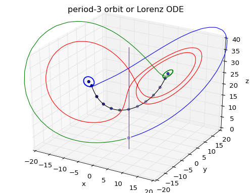
Compute all periodic orbits of the Lorenz ODE up to period 4 and produce a plot for each, like these.

Use the classic parameter values  . Use whatever software system you like (Matlab, Julia, Mathematica, C, Fortran, whatever). Compute the orbits with these steps.
Step 1: Plot the three unstable equilibria with dots. Compute and plot the stable manifold of the origin and a portion its unstable manifold as shown (magenta for stable manifold, blue and green for stable).
Step 2: Plot the pseudo-Poincare section given by the curve 

for  . This 1d curve lies pretty nearly on the attracting set. (I got it by guessing the right form and setting the constants by trial and error). Parameterize this curve numerically by
  so that is
  at the end points and zero at the center (simplest strategy: let
  ).
).
Step 3: Let  be the return map of onto itself (hand-wavey, because trajectories starting on the curve don't actually come back exactly to ). Create a table of
data of
be the return map of onto itself (hand-wavey, because trajectories starting on the curve don't actually come back exactly to ). Create a table of
data of  pairs by numerical integration of points starting on the curve. Make a plot of
  using this numerical data.
Step 4: Fit a function to the the numerical data from above. A piecewise polynomial with three or four terms should do. Plot this on top of your numerical values.
Step 5: Plot  versus along with the diagonal to get an estimate of the value of the period-n orbit. Then use the corresponding
  values as an initial guess for a periodic orbit.
Step 6: Compute the periodic orbit, either approximately by adjusting until the trajectory very nearly lands back on its starting point, or better, by setting up a function  which maps forward time
  under the Lorenz dynamics, using numerical integration, and then applying a nonlinear numerical solution method to find a zero of the function
  .
.
Choice 2: The Rössler system
Compute the first four or five periodic orbits of the Rössler system

with  and
and  . A long trajectory of the Rössler system looks like this
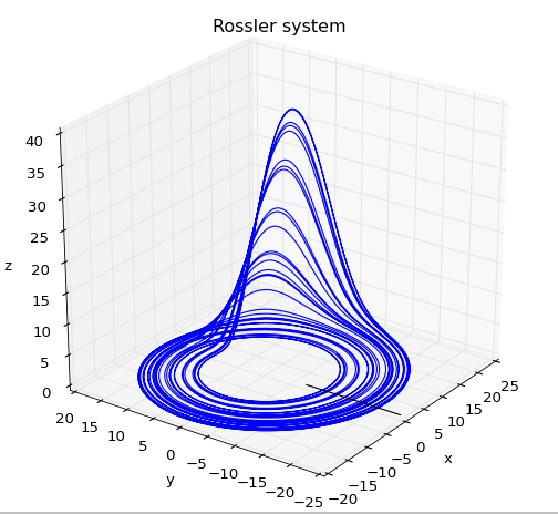
Step 1: Find the equilibria and the eigenvalues of the equilibrium near the origin. What is the period of the revolution about the equilibrium and the growth factor per revolution?
Step 2: Let the  plane define a Poincare section. Trajectories crossing this plane with
  increasing will have
  very nearly zero, so the value of
  at serves as a good coordinate for a 1d return map. The above picture has a black line drawn from
  with
with  . Figure out a good parameterization to
 ![$\eta = [0,1]$](/dokuwiki/lib/exe/fetch.php?media=wiki:latex:/img0095ac2effb28a0bd01620f3f523d87f.png "Math") of a subset of this line and construct a 1d return map by integrating trajectories from points on it.
of a subset of this line and construct a 1d return map by integrating trajectories from points on it.
Step 3: Approximate the numerical return map from step 2 with an analytic function, then use the fixed points of higher-order iterates of the return map to get initial guesses for periodic orbits.
Step 4: Find periodic orbits numerically by solving a nonlinear equation as described in step 6 for Lorenz.
