Important matlab commands: linspace, meshgrid, pcolor, surf, contour, surfc, contourf, quiver, mesh, load, subplot, pcolor, shading.

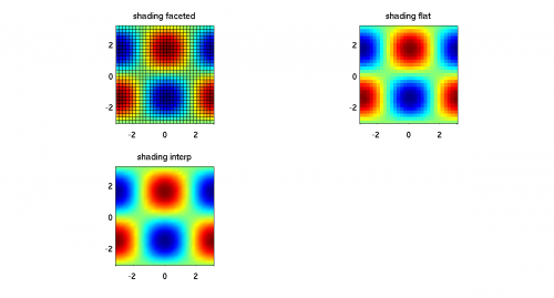
Skim the Matlab documentation for linspace, meshgrid, and pcolor. Create a 2D mesh from −π to π with 30 points in both the x and y directions. Then for each position in the mesh let z = cos(x) sin(y). Use pcolor, axis equal, and axis tight to generate this figure:

But don't you hate those ugly black lines? You can get rid of them with the shading command. Use subplot and the shading command to generate this figure:

Create a 2D mesh from −π to π with 20 points in both the x and y directions, let z = cos(x) sin(y) pointwise, and then recreate this figure using the surf and colorbar commands.

Create a 2D mesh from −10 to 10 with 100 points in both the x and y directions, let and z = 5 sin(r)/r. Then recreate Figure 4 using the surf and shading commands.

Create a 2D mesh from −π to π with 100 points in both the x and y directions and then recreate Figure 5, using the functions z = cos(x/2) cos(y/2), z = sin(x) cos(y/2), z = cos(x/2) sin(y), and z = sin(x) sin(y).

Enter the following code into a script file, save the figure produced as a '.jpg' or '.png' image, and include it with your project. What does the image produce? What is the role of the 'C' variable?

[phi,theta] = meshgrid(linspace(0,2*pi,100));
X=(cos(phi) + 3) .* cos(theta);
Y=(cos(phi) + 3) .* sin(theta);
Z=sin(phi);
C=sin(3*theta);
surf(X,Y,Z,C)
shading interp

The function

is a rough scale model of a pair of small mountains named Monte Sol and Monte Luna on the outskirts of Santa Fe, New Mexico. Monte Sol, the bigger of the two mountains is about 200 meters high above the plain, so the scale is 1 = 100 meters.

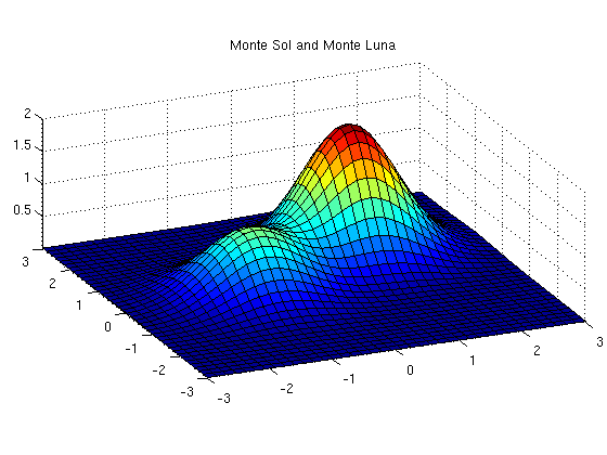
(a) Reproduce the above surface plot in Matlab.

(b) In a gentle rainstorm, water will flow down the mountains in the direction of steepest descent, i.e. along the negative of the gradient of . Find the gradient of using elementary calculus, then make an plot with both contours of the mountain height and a quiver plot showing the direction of flow of rainwater.

Draw a Klein bottle in Matlab. Feel free to search the web, but understand whatever you use.

Attribution: This lab is adapted from Prof.Mark Lyon's Math 445 Advanced Graphics lab, which is adapted from Octave demos at http://yapso.sourceforge.net/demo/demo.html.