% In honor of Yitang (Tom) Zhang's proof of the boundedness of gaps 
% between primes, and of his MacArthur Fellowship announced yesterday,
% let's use Matlab to find the twin primes between 1 and N. This will
% demonstrate a number of logical array operations
 
% Matlab's 'prime(N)' function will return the prime numbers less than
% or equal to N. Let's first set N=31 to get a small set of primes, so
% we can see in detail how the operations work. 
 
>> p = primes(35)
p =
     2     3     5     7    11    13    17    19    23    29    31
 
% Twin primes are consecutive prime numbers that differ by 2. 
% To find twin primes, we'll compare two offset subvectors of p
 
>> firstprime = p(1:end-1)
firstprime =
     2     3     5     7    11    13    17    19    23    29
 
>> nextprime = p(2:end)
nextprime =
     3     5     7    11    13    17    19    23    29    31
 
% Now perform a logical array operation on these subvectors. 
% Recall that == is Matlab's equality test (whereas = is assignment).
% x == y for vectors x and y will perform an elementwise equility 
% test and return a vector of 0's and 1's, with 1's marking elements
% that are equal. 
 
>> istwin = (firstprime + 2 == nextprime)
istwin =
     0     1     1     0     1     0     1     0     0     1
 
 
% Matlab's 'find' command will return the indices of the nonzero elements
% of a vector. Thus we can use the result of 'find(istwin)' to index back 
% into the list of primes p and extract the first prime of each twin prime 
% pair.
 
>> indices = find(istwin)
indices =
     2     3     5     7    10
 
>> p(indices)
ans =
     3     5    11    17    29
 
>> p(indices+1)
ans =
     5     7    13    19    31
 
% Voila! p(indices) gives us the first prime of each twin prime pair.
% indices+1 adds 1 to each element of indices, so p(indices+1) gives
% the second prime in each twin prime pair.
 
% Ok, that was the long-winded way to do it. Now let's find all twin 
% primes less than N=1000, as compactly as possible. 
 
>> p = primes(1000);
>> p(find(p(1:end-1) + 2 == p(2:end)))
 
ans =
  Columns 1 through 13
     3     5    11    17    29    41    59    71   101   107   137   149   179
  Columns 14 through 26
   191   197   227   239   269   281   311   347   419   431   461   521   569
  Columns 27 through 35
   599   617   641   659   809   821   827   857   881
 
>> p(find(p(1:end-1) + 2 == p(2:end))+1)
 
ans =
  Columns 1 through 13
     5     7    13    19    31    43    61    73   103   109   139   151   181
  Columns 14 through 26
   193   199   229   241   271   283   313   349   421   433   463   523   571
  Columns 27 through 35
   601   619   643   661   811   823   829   859   883
 
% That output is a little hard to read, so let's assign the results into a matrix
% with two columns, each row consisting of a twin prime pair. Note the ', which 
% transposes the row-vector lists of primes from above into column vectors for
% insertion into a matrix P. Note also that I don't even need to allocate P with 
% 'zeros' --Matlab figures out how big P should be as we go along. 
 
P(:,1) =  p(find(p(1:end-1) + 2 == p(2:end)))';
P(:,2) =  p(find(p(1:end-1) + 2 == p(2:end))+1)';
 
% The twin primes less than 1000
>> P
P =
     3     5
     5     7
    11    13
    17    19
    29    31
    41    43
    59    61
    71    73
   101   103
   107   109
   137   139
   149   151
   179   181
   191   193
   197   199
   227   229
   239   241
   269   271
   281   283
   311   313
   347   349
   419   421
   431   433
   461   463
   521   523
   569   571
   599   601
   617   619
   641   643
   659   661
   809   811
   821   823
   827   829
   857   859
   881   883
 
 
% Thus ends our homage to Yitang 'Tom' Zhang. I encourage you to 
% view Tom's video on the MacArthur Foundation website. 

% =======================================================================
% Now a couple examples of summing series, as compactly as possible
% Let's sum 1 + 1/2 + 1/4 + 1/8 + .... The nth term is 1/2^n or (1/2)^n, 
% 
% Can get the first N terms with elementwise array operations
 
>> n=0:6
n =
     0     1     2     3     4     5     6
 
>> (1/2).^n
ans =
    1.0000    0.5000    0.2500    0.1250    0.0625    0.0312    0.0156
 
>> sum((1/2).^n)
ans =
    1.9844
 
>> format long
>> sum((1/2).^n)
ans =
   1.984375000000000
 
% Even more compactly, and now summing the first eleven terms, twenty-one terms, etc.
>> sum((1/2).^[0:10])
ans =
   1.999023437500000
 
>> sum((1/2).^[0:20])
ans =
   1.999999046325684
 
>> sum((1/2).^[0:30])
ans =
   1.999999999068677
 
>> sum((1/2).^[0:40])
ans =
   1.999999999999091
 
>> sum((1/2).^[0:50])
ans =
   1.999999999999999
 
>> sum((1/2).^[0:60])
ans =
     2

% Load datafile 'data1.asc' into matlab with 'load' command
>> D = load('data1.asc'); 
 
% extract first column as variable x, second as y
>> x = D(:,1)
xdata =
  -73.6780
  -39.7800
   -5.7090
    7.2455
   21.2370
   53.6940
   61.2940
   66.5520
   70.4650
   98.6480
 
>> ydata = D(:,2)
ydata =
   55.5800
   38.9020
   22.1390
   15.7650
    8.8812
   -7.0872
  -10.8270
  -13.4140
  -15.3390
  -29.2050
 
% Plot y versus x for the data, with circles on the datapoints. 
>> plot(xdata, ydata, 'mo-')
>> xlabel('x')
>> ylabel('y')
>> grid on

% It's a straight line on a linear plot, so the functional relation is y = mx + b. 
% Hmmm, the slope is negative, dropping about 1 in y for every 2 in x. So I'll 
% guess a slope of m = -1/2. The intercept with the y axis looks to be about 18. 
% Making a quick guess at that the relation is y = -0.5 x + 18 and plot the guess
% together with the data
 
>> x = linspace(-80,100, 10);
>> y = -0.5 * x + 18;
>> plot(xdata, ydata, 'mo-', x, y, 'b.-')
>> xlabel('x'); ylabel('y')

% Wow, that's a great guess! But the slope is a little too negative, and the
% y-intercept a little low. Try y = -0.49 x + 18.5. And this time let's just put
% the expression for y into the plot command, with the labeling commands following
% on the same line, so that we can regenerate the plot with different constants 
% quickly by making small changes to a single command line.
 
>> plot(xdata, ydata, 'mo-', x, -0.49 * x + 18.5, 'b-'); xlabel('x'); ylabel('y'); grid on;

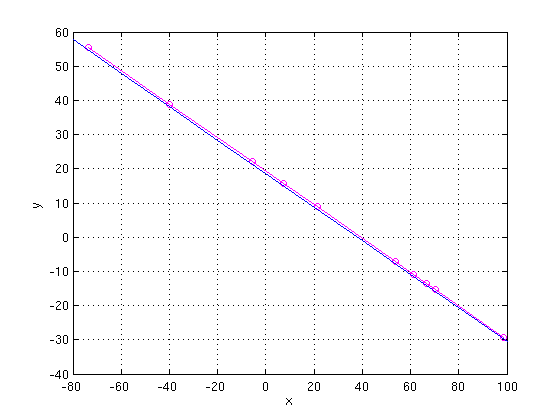
% Even better! The slope looks just right but our guess is still a little low.
% Raise the y intercept up to 19.
 
>> plot(xdata, ydata, 'mo-', x, -0.49 * x + 19, 'b-'); xlabel('x'); ylabel('y'); grid on;

% Perfect! So the functional relation between y and x is y = -0.49 x + 19

% Load the next data file and try to figure out its y = f(x) relation. 
>> D = load('data3.asc');
>> xdata = D(:,1);
>> ydata = D(:,2);
>> plot(xdata, ydata,'mo-'); xlabel('x'); ylabel('y'); grid on

% That looks exponential, so graph y logarithmically
>> semilogy(xdata, ydata, 'mo-'); xlabel('x'); ylabel('y'); grid on

% Great! It's a straight line with y graphed logatithmically, so the relation is
% of the form 
%   log10 y = m x + b,   or equivalently
%         y = 10^(mx+b), or equivalently
%         y = c 10^(mx)
% for some constants m and c. let's take rough guesses, judging from the plot.
%
% m is the slope in log10 y versus x. log10 y drops from 2 at x=10 to about 1 at x=20.
% So m looks to be about -1/10, (rise of -1 over run of 10). You can get the constant c
% by estimating the value of y at x=0. That looks to be about c=400. So let's give
% y = 400 10^(-0.1 x) a try.
 
>> x = linspace(-20, 50, 10);
>> semilogy(xdata, ydata,'mo-', x, 400*10.^(-0.1*x)); xlabel('x'); ylabel('y'); grid on

% Not too shabby. But the slope is a little too negative and y is too low at x=0. 
% A few iterations of adjusting the constants gives
 
>> semilogy(xdata, ydata,'mo-', x, 700*10.^(-0.085*x)); xlabel('x'); ylabel('y'); grid on

% so the functional form is y = 700 * 10^(-0.085 x). 
 
% Don't ask me why Matlab keeps changing the grid lines on the logarithmic plots...