How do you figure out the path of a object whose velocity is a given function of its position ? I.e., given that

for some known function , along with an initial position , how do you solve for the path ? (Note that here and should be considered vector-valued quantities. I'm leaving out the arrows on top to reduce clutter.)

The above equation is an ordinary differential equation. MATH 527 Differential Equations is all about finding solutions to such equations in closed form. Here we will use numerical solution methods to find approximate numerical solutions.

To make things concrete, let's solve the following problem. Given the 2D inviscid flow around a cylinder from the last lecture, what would be the path of a small particle starting at position , shown below as a red circle?

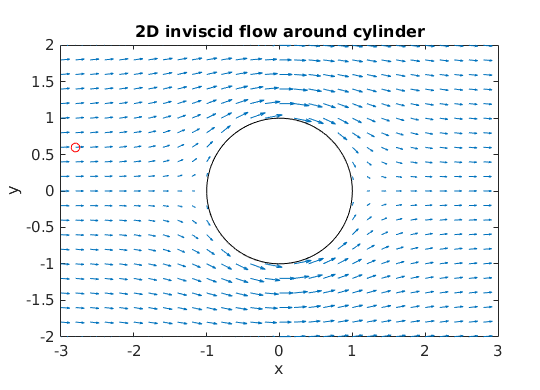
Here's the code for plotting the 2D inviscid cylinder flow. The line x = [-3.8, 0.6]; plot(x(1), x(2), 'ro'); plots the dot. The problem now is to compute and plot the particle as it's advected along by the fluid velocity field , where

and where are the polar coordinates of the vector position .

Write Matlab code that plots the motion of the particle, in discrete steps, using the forward-Euler timestepping formula

This equation says, essentially, that the distance a particle at position moves in a small time interval is given by the product of and the velocity of the fluid at that point.

Here's some Matlab code that implements the forward Euler timestepping with a simple for loop.

%%%%%%%%%%%%%%%%%%%%%%%%%%%%%%%%%%%%%%%%%%%%%%%%%%%%%%%%%%%%%%%
% Simulate a particle moving through the inviscid cylinder flow
% using forward Euler time-stepping 
%
%    x(t + dt) = x(t) + dt*v(x(t));
% 
% Integrate from t=0 to t=9 in small steps of length dt (say dt=0.1)
% That is, find the path x(t) for 0 <= t <= 9. 
 
T = 9;
dt = 0.4;
Nsteps = round(T/dt);
 
x = [-2.8; 0.6];           % initial position of particle
 
hold on;
 
for n=1:Nsteps;
  plot(x(1), x(2), 'ro')
  x = x + dt*v(x);         % update position using forward euler
  pause
end

Note that the above code calls a function v(x), which is defined in the Matlab function file v.m

v.m

function dxdt = v(x)
  % return velocity vector v(x) for cylinder flow at position x
  V0 = 1;
  a  = 1;
 
  r = sqrt(x(1)^2 + x(2)^2);
  theta = atan2(x(2),x(1));
 
  dxdt = [V0*(1 - a^2/r^2 * cos(2*theta));
         -V0*a^2/r^2 * sin(2*theta)];
 
end

Note that the trajectory computed here is not very accurate. The fluid velocity field is symmetric in , so the particle should exit the box at the same value it had when it entered. The problem is we chose quite a large time step , and forward-Euler is only 1st-order accurate (error scales as ). In the next problem, we'll reduce the time step to and get a more accurate solution –though still not as good as the 4th-order accurate ode45 function.

Write Matlab code that plots the path of the particle as a red curved line. To do this we need to save the sequence of values in a matrix, and then plot the rows of that matrix as a line.

T = 10;      % integrate from t=0 to T=10, i.e 0 <= t <= 10
dt = 0.01;   % 
Nsteps = round(T/dt); 
 
X = zeros(2,Nsteps);  % stores sequences of x(t) values as cols in a matrix
X(:,1) = [-2.8; 0.1]; % initial position of particle
 
for n=1:Nsteps
  X(:,n+1) = X(:,n) + dt*v(X(:,n));  % forward euler time stepping
end
 
plot(X(1,:), X(2,:), 'r-');
 
axis equal
axis tight
xlim([-3,3])
ylim([-2,2])

Write Matlab code that plots the path of the particle as a red curved line, using Matlab's ode45 function to do the time-integration.

% use Matlab's ode45 function to do the time integration of 
% dx/dt = v(t, x)
 
T = 10;           % integrate from t=0 to T=10
x0 = [-2.8; 0.6]; % initial position of particle
 
[t, x] = ode45(@v, [0 T], x0);  % computes x(t) at given values of t
 
plot(x(:,1), x(:,2), 'r-');
 
axis equal
axis tight
xlim([-3,3])
ylim([-2,2])

Matlab's ode45 function requires an ODE of the form , so we have to add a t argument to our v function

v.m

function dxdt = v(t, x);
  % compute 2D inviscid cylinder velocity as function of x
  % input: vector x has x(1) = x coord, x(2) = y coord
 
  V0 = 1;  % scale of velocity
  a  = 1;  % radius of circle
 
  % compute polar coordinates
  r = sqrt(x(1)^2 + x(2)^2); 
  theta = atan2(x(2), x(1));        
 
  dxdt = [V0*(1 - (a/r)^2 * cos(2*theta)) ; 
         -V0*(a/r)^2 * sin(2*theta)];
 
end

This produces a plot very like the one for Problem 3.

Draw a number of particle paths starting with a number of values and .

% use Matlab's ode45 function to do the time integration of 
% dx/dt = v(t, x)
 
T = 10;                           % integrate from t=0 to T=10
 
for y = -2:0.4:2                  % loop over different y values
 
  x0 = [-2.8; y];                 % set initial position of particle
 
  [t, x] = ode45(@v, [0 T], x0);  % compute x(t) over range 0 <= t <= T
 
  plot(x(:,1), x(:,2), 'r-');     % plot the path
 
end